I’ve long admired the work of Ed Fairburn. In many of his pieces he draws on old topographic maps, using the contour lines to build up stunning portraits. For Abi’s birthday I thought I’d try to do something similar with a region of the Moon that Abi and I have spent a lot of time analyzing together. I considered commissioning Ed directly as he’s worked with lunar maps in the past, but as far as I’m aware there aren’t any good topographic maps of the area I’m interested in – at least not at the resolution I was aiming for. This is meant to serve as a little tutorial on how I achieved this effect.

Using terrain models

I pulled a digital terrain model (DTM) constructed from measurements captured by the Lunar Orbiter Laser Altimeter. imbrium.mit.edu has a great collection of lunar DTMs for use at a wide range of resolutions. This time we want the gridded data records (GDRs) because the rasters will be easier to work with.

From there we can pull out the region we want. If you already know the appropriate coordinates in the projection that your map is in, using gdalwarp is probably the simplest option. Otherwise you can use this little python function to convert from lat/lon coordinates to whatever projection your map is in:

 1
 2
 3
 4
 5
 6
 7
 8
 9
10
11
12
13
14
15
16
17
18
19
20
21
22
23
24
25
26
27
28
29
30
31
32
33
34
35
36

from osgeo import osr, gdal

# Latitude and longitude expressed in degrees.
# Width and height expressed in meters.
def load_dtm(lat, lon, width, height):
  dataset = gdal.Open(DTM_FILENAME)
  # srs contains the coordinate system  of the DTM
  # srs_lat_lon contains the lat/lon coordinate system
  # coordinate_transform converts from lat/lon to the DTM coordinates
  srs = osr.SpatialReference()
  srs.ImportFromWkt(dataset.GetProjection())
  srs_lat_lon = srs.CloneGeogCS()
  coordinate_transform = osr.CoordinateTransformation(srs_lat_lon, srs)
  x, y, _ = coordinate_transform.TransformPoint(lon, lat)

  # convert x/y into pixel coordinates
  raster = dataset.GetRasterBand(1)
  image_transform = dataset.GetGeoTransform()
  x_origin = image_transform[0]
  y_origin = image_transform[3]
  pixel_width = image_transform[1]
  pixel_height = -image_transform[5]
  img_x = int((x-x_origin)/pixel_width + 0.5)
  img_y = int((y_origin-y)/pixel_height + 0.5)

  # Read into a numpy array
  left = img_x - int(width / pixel_width)
  right = img_x + int(width / pixel_width)
  top = img_y - int(height / pixel_height)
  bottom = img_y + int(height / pixel_height)
  data = raster.ReadAsArray(left, top, right-left, bottom-top)

  # Imbrium DTMs have elevations multiplied by 2
  # Multiplying by raster.GetScale() undoes this
  data = data * raster.GetScale()
  return data

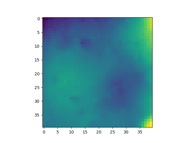
After this I used scipy.ndimage.zoom and scipy.ndimage.gaussian_filter to increase the working resolution and reduce pixelation artifacts in the contour lines.

Generating halftone pattern

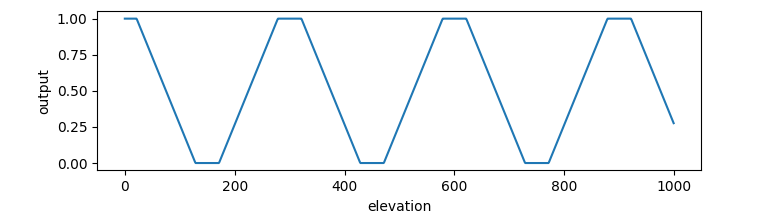
For the halftone effect, we want regions close to contours lines to be closer to black and the areas far from the contour lines to be lighter. To achieve this we’ll use a “ping-pong” function that bounces between 0 (at contour lines) and 1 (exactly between two contour lines).

1
2
3
4

contour_distance = 3
data = data % contour_distance
data -= contour_distance / 2
data = np.abs(data) / (contour_distance / 2)

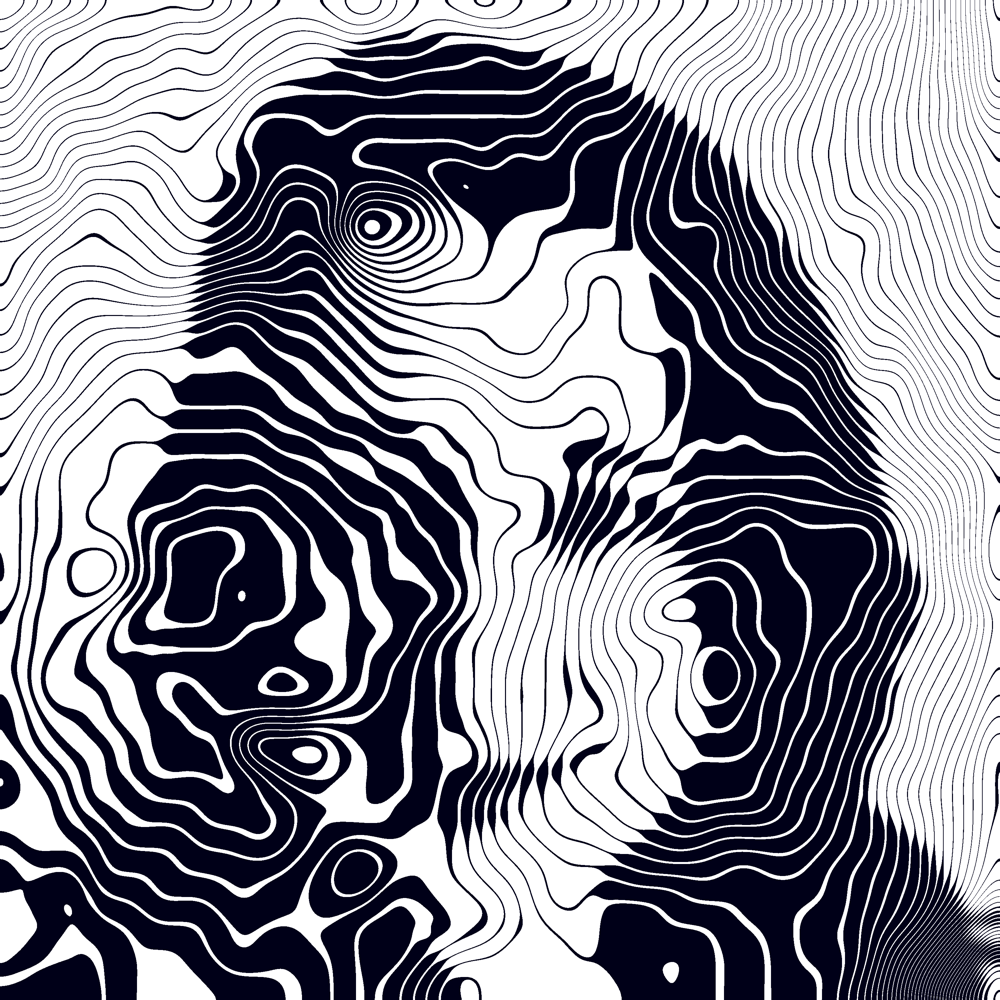
Because I wanted to make sure that contours never completely disappeared nor got completely filled in, I made sure to overshoot the [0-1] range a bit and then clamped it so the elevation function ends up looking a bit like:

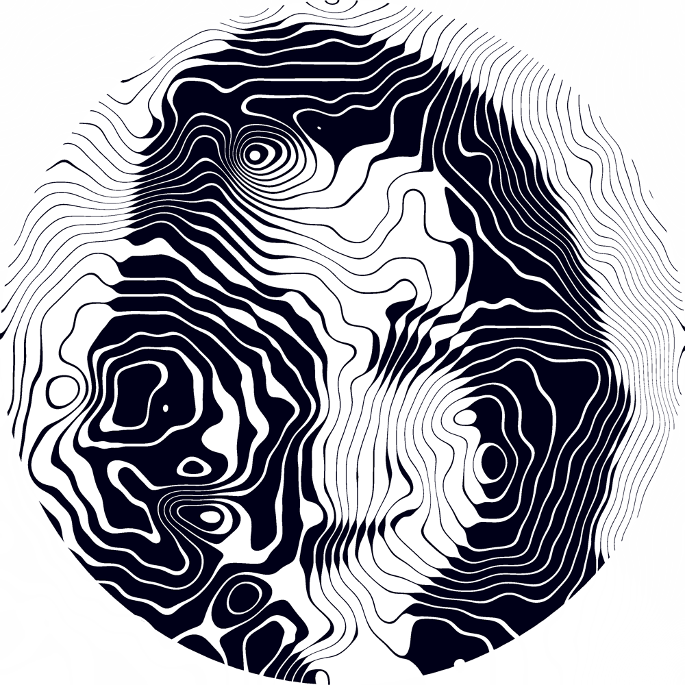
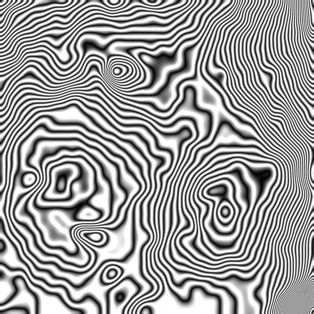
And you should end up with something more or less like this trippy pattern:

Applying to an image

After generating the halftone pattern, we can apply it to our desired image. This can be done by either multiplying the pixel luminosities, though I found the most success through an arithmetic mean. After applying a threshold you should be done!

 1
 2
 3
 4
 5
 6
 7
 8
 9
10
11
12

from PIL import Image

base_image = Image.open(BASE_IMAGE_FILENAME)
base_image = base_image.convert('L') # convert to grayscale
base_image = np.asarray(base_image)
result = (data * 255 + base_image) / 2 # arithmetic mean
result = result < 140 # apply threshold

# convert back to image
result = result * 255
result = Image.fromarray(np.uint8(result))
result.save('result.png')

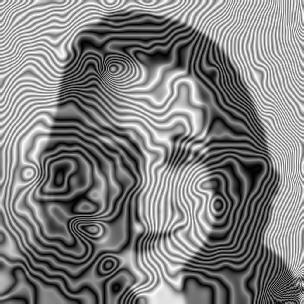
To quickly hack in some basic anti-aliasing, I simply generated the image 3 times larger than needed and downsized afterwards. This caused some memory issues on my laptop but was so easy to implement that I didn’t bother doing anything fancier. I also applied a circular mask to the result to hide that region in the bottom right where the contours are a bit too close together for my liking.

Wrapping up

A coworker recommended I use Whitewall to print, and I have to say I was quite happy with their service. They said it would arrive in 9 business days, but it showed up in less than 2, and the quality of the print was more than suitable.

I’m very happy with how this turned out, though with there was an enormous amount of fiddling necessary to produce decent results and I feel it still lacks a lot of the compositional finesse that Ed Fairburn is able to pull off. If you’re interested in a piece in this style, but want a better result without tweaking variables for hours, I highly recommend you look into commissioning some of Ed’s incredible work.